Abstract
This research investigates the profound impact of land pollution on soil degradation, stemming from human-made (xenobiotic) chemicals and alterations in soil composition. The framework explains a comprehensive nonlinear fractal fractional order eco-epidemic model, delineating four compartments: Susceptible soil (S), Polluted soil (P), Remediation or recycling of polluted soil (T), and Recovered soil (R). The study rigorously establishes the non-negative and unique existence of solutions using the fixed point theorem while analyzing the local and global stability of equilibrium points under pollution-free equilibrium and pollution extinct equilibrium. Dula’s criterion confirms periodic orbits, while categorizing changes in secondary reproduction numbers provides crucial insights into pollution dynamics, enhancing our understanding of system dynamics. Local and global sensitivity analyses, employing forward sensitivity and the Morris Method, yield essential findings for informed decision-making. Additionally, Adams-Bashforth's method is employed to approximate solutions, facilitating the integration of theoretical concepts with practical applications. Supported by numerical simulations conducted in MATLAB, the study offers a nuanced understanding of parameter roles and validates theoretical propositions, ultimately contributing valuable insights to environmental management and policy formulation.
Keywords
Soil Pollution, Fractional Order Model, Stability, Adams Bashforth Technique, Lyapunov Function, Sensitivity Analysis
1. Introduction
Mathematical modeling serves as an indispensable tool for comprehending the dynamic mechanisms underlying the spread of infectious diseases and devising effective strategies to mitigate economic losses. A pivotal achievement in mathematical epidemiology lies in the formulation, prediction, and identification of disease control measures through rigorous mathematical expressions. Traditionally, epidemiological models have compartmentalized a constant population into three categories: susceptible, infectious, and recovered. The evolution of these models has seen the inclusion of various compartment classes, adapting to the variation of available descriptive information. In the budding stages of research, the discourse predominantly revolved around integer-order differential equations. However, recent strides in the field have witnessed the emergence of fractional-order mathematical modeling, playing a substantial role in addressing a diverse array of challenges in engineering, epidemiology, ecology, and biology. Fractional calculus, as a generalization where the conventional integer order gives way to a fractional order, provides a more varied approach
| [21] | S. B. Kurniawan, “Bioprocess of Trivalent Chromium using Bacillus subtilis and Pseudomonas putida”, Department of Environmental Eng., FTSLK ITS Surabaya, 2016. |
| [22] | Sherene T., “Heavy Metal status of soils in Industrial Belts of Coimbatore District, Tamil Nadu”, Nature environment and pollution technology, Vol. 8, No. 3, pp. 613-618, 2009. |
| [23] | S. S Askar, Dipankar Ghosh, “A fractional order SITR Mathematical model for forecasting of transmission of Covid 19 of India with lockdown effect”, Results in Physics 24, 104067, 2021. |
| [24] | Subrata Paul and Animesh Mahata, “Dynamics of SIQR epidemic model with fractional order derivative”, Partial differential equation in applied mathematics, vol. 5, 100216, 2022. |
| [25] | V. Lakshmikantham and A. S. Vatsala, “Theory of fractional differential inequalities and applications,” Communications in Applied Analysis, vol. 11, pp. 395–402, 2007. |
[21-25]
. Notably, as the order approaches one, the solution of the fractional order converges to that of the integer order system. The fractional order system introduces two critical properties—the memory property and hereditary property—which are not adequately captured by any integer order system. These properties contribute to a more accurate representation of real-world phenomena. The fractional order system aligns well with theoretical descriptions of various mechanisms, offering a sophisticated understanding of dynamics
| [26] | V. Lakshmikantham and A. S. Vatsala, “Basic theory of fractional differential equations,” Nonlinear Analysis: Theory, Methods & Applications, vol. 69, no. 8, pp. 2677–2682, 2008. |
| [28] | Wu, Jianyong, et al. "Sensitivity analysis of infectious disease models: methods, advances and their application." Journal of The Royal Society Interface 10.86(2013): 20121018. |
| [29] | Y. Li, Y. Chen and I. Podlubny, “Stability of fractional-order nonlinear dynamic systems: Lyapunov direct method and generalized Mittag-Leffler stability,” Computers & Mathematics with Applications, vol. 59, no. 5, pp. 1810–1821, 2010. |
[26, 28-29]
. Over the last few decades, various types of fractional calculus, including Riemann–Liouville, Caputo, Atangana–Baleanu, Caputo–Fabrizio, Katugampola, Hadamard, etc., have been introduced extensively to scrutinize the dynamics of epidemic models. This ongoing exploration holds the promise of refining our capacity to model and comprehend intricate systems across diverse fields.
| [1] | A. Kilbas, H. M. Srivastava and J. J. Trujillo, “Theory and Applications of Fractional Differential Equations”, Elsevier, Amsterdam, The Netherlands, 2006. |
| [2] | Babakhani and V. Daftardar-Gejji, “Existence of positive solutions of nonlinear fractional differential equations”, Journal of mathematical analysis and applications, vol. 278, no. 2, pp. 434-442, 2003. |
| [3] | C. F. Li, X, N. Luo, Y. Zhou and J. J, “Existence of positive solution of the boundary value problem for nonlinear fractional differential equations”, Computer and Mathematics with applications, vol. 59, pp. 1363-1375, 2010. |
| [4] | D. Kumar and J. Singh, “Application of Homotopy analysis transform method to fractional biological population model”, Romanian reports physics, vol. 65, no. 1, pp. 63-75, 2013. |
| [5] | Elhia, M., Balatif, O., Boujallal, L., & Rachik, M. Optimal control problem for a tuberculosis model with multiple infectious compartments and time delays. An International Journal of Optimization and Control: Theories & Applications (IJOCTA), 11(1), 75-91. (2021). |
| [6] | Evirgen, Fırat, et al. "Real data-based optimal control strategies for assessing the impact of the Omicron variant on heart attacks." AIMS Bioengineering 10.3 (2023). |
[1-6]
Subtrapaul, et.,
| [24] | Subrata Paul and Animesh Mahata, “Dynamics of SIQR epidemic model with fractional order derivative”, Partial differential equation in applied mathematics, vol. 5, 100216, 2022. |
[24]
proposed the dynamical behavior of the COVID-19 epidemic SIQR model in terms of fractional order. S. S. Askar, and Dipankar Ghosh,
| [23] | S. S Askar, Dipankar Ghosh, “A fractional order SITR Mathematical model for forecasting of transmission of Covid 19 of India with lockdown effect”, Results in Physics 24, 104067, 2021. |
[23]
studied the h-stability of the Caputo fractional order differential equation by using some fractional comparison principle and the Lyapunov direct method. Mukherjee D, and Mondal R,
| [15] | Mukharjee D and Mondal R, “Dynamical analysis of a Fractional Order Prey-Predator system with reserved area”, J Fract Calc Appl 11, 54-69, 2020. |
[15]
deal with the fractional order prey-predator model of the dynamical system for the reserved area and present the numerical analysis of hopf-bifurcation. Zizhen Zhang et al.,
| [30] | Zhang, Zizhen, et al. "Dynamics of a fractional order mathematical model for COVID-19 epidemic." Advances in Difference Equations 2020. 1(2020): 1-16. |
[30]
formulated and analyzed the dynamics of the COVID-19 epidemic models with an isolated class of fractional order. Many researchers proposed many models in eco-epidemiology and analyzed the various stability properties, existence, and non-negativity of the solution
| [7] | F. Haq, K. Shah, G. Rahman and M, Shahzad, “Existence and uniqueness of positive solutions to boundary value problem of fractional differential equations”, Sindh Univ. Res. Jour, vol. 48, no. 2, pp. 451-456, 2016. |
| [8] | Evirgen, F., Ucar, E., ÖZDEMIR, N., Altun, E., & Abdeljawad, T. (2023). The impact of nonsingular memory on the mathematical model of Hepatitis C virus. Fractals, 2340065. |
| [9] | F. Haq, K. Shah, G.-U. Rahman and M. Shahzad, “Numerical analysis of fractional order model of HIV-1 infection of CD4+ T cells”, Computational methods for differential Equations, vol. 5, no. 1, pp. 1-11, 2017. |
| [10] | Fazal Haq and Muhammad Shahzad, “Numerical Analysis of Fractional Order Epidemic Model of Childhood Disease”, Discrete Dynamics in Nature and Society, vol. 2017, Article Id 4057089, pp. 7, 2017. |
| [11] | Hamou, Abdelouahed Alla, et al. "Analysis and dynamics of a mathematical model to predict unreported cases of COVID-19 epidemic in Morocco." Computational and Applied Mathematics 41.6 (2022): 289. |
| [12] | Ipung Fitri Purwanti and Tesya Paramita Putri, “Treatment of Chromium Contaminated Soil using Bioremediation”, AIP Conference Proceeding, 1903, 040008, 2017. |
| [13] | Kashyap, A. J., Bhattacharjee, D., & Sarmah, H. K. (2021). A fractional model in exploring the role of fear in mass mortality of pelicans in the Salton Sea. An International Journal of Optimization and Control: Theories & Applications (IJOCTA), 11(3), 28–51. https://doi.org/10.11121/ijocta.2021.1123 |
| [14] | Liao, Teh-lu. "Adaptive synchronization of two Lorenz systems." Chaos, Solitons & Fractals 9.9 (1998): 1555-1561. |
| [15] | Mukharjee D and Mondal R, “Dynamical analysis of a Fractional Order Prey-Predator system with reserved area”, J Fract Calc Appl 11, 54-69, 2020. |
[7-15]
. Numerical approximation of the proposed model has been done by the Rung-Kutta method, Taylor series method, Adams Bashforth and Adams Moulton method, Adomain and Laplace Adomian decomposition method, Homotopy method and generalization of homotopy method
| [14] | Liao, Teh-lu. "Adaptive synchronization of two Lorenz systems." Chaos, Solitons & Fractals 9.9 (1998): 1555-1561. |
[14]
. In this work, the Laplace Adomain decomposition method is used to study the approximate solution of the proposed model. The Laplace Adomian decomposition method was introduced by Adomian in 1980. This is a very effective method to find the explicit and numerical solution to the physical problem of ordinary and partial differential equations with nonlinear initial and boundary conditions. It can also be used to study many deterministic, stochastic diffusion models with and without delay. There is no perturbation and linearization is required and also no extra memory is required to solve this problem which is the main advantage of the method
| [16] | Muhammad Rafiq and Javaid Ali,“Numerical Analysis of a bi-model covid-19 SITR model”, Alexandria Engineering Journal, vol. 61, pp. 227-235, 2022. |
| [17] | Noor Badshah and Haji Akbar, “Stability analysis of fractional order SEIR model for malaria disease in Khyber Pakhtunkhwa”, Demonstratio Mathematica, vol. 54, pp. 326-334, 2021. |
| [18] | Nuri Ozalp and Elif Demiric, “A fractional order SEIR model with vertical transmission”, Mathematics and computer modeling, 54, pp. 1-6, 2011. |
| [19] | O. D. Makinde, “Adomain decomposition approach to a SIR epidemic model with constant vaccination strategy”, Applied Mathematics and Computation, vol. 184, no. 2, pp. 842-848, 2007. |
| [20] | Ozdemir, Necati, Esmehan Uçar, and Derya Avcı. "Dynamic analysis of a fractional svir system modeling an infectious disease." Facta Universitatis, Series: Mathematics and Informatics (2022): 605-619. |
[16-20]
.
Sensitivity analysis (SA) is increasingly popular in developing more efficient models, requiring reliable statistical and mathematical methods to enhance modeling accuracy. SA serves various purposes, including developing decisions or recommendations, communicating, understanding, or quantifying systems, and refining models. During model development, SA verifies validity or accuracy, simplifies and calibrates weak processes or missing data, and identifies important parameters for further studies. These applications highlight SA's versatility and importance in refining models and optimizing decision-making processes.
The main aim of this paper is to study the mathematical model of Caputo fractional order soil pollution. Soil is the main requirement for living and non-living organisms. In the case of contamination of soil as such oil spill, excess use of heavy metals, and inorganic fertilizer, the soils are polluted. All polluted soil contains compounds that include metals, inorganic iron salts (phosphates, carbonates, sulfates, nitrates), and organic compounds (lipids, DNA, fatty acids, alcohol). These compounds are mainly entered through soil microbial activity and decomposition of organisms (animals and plants)
| [10] | Fazal Haq and Muhammad Shahzad, “Numerical Analysis of Fractional Order Epidemic Model of Childhood Disease”, Discrete Dynamics in Nature and Society, vol. 2017, Article Id 4057089, pp. 7, 2017. |
| [17] | Noor Badshah and Haji Akbar, “Stability analysis of fractional order SEIR model for malaria disease in Khyber Pakhtunkhwa”, Demonstratio Mathematica, vol. 54, pp. 326-334, 2021. |
| [18] | Nuri Ozalp and Elif Demiric, “A fractional order SEIR model with vertical transmission”, Mathematics and computer modeling, 54, pp. 1-6, 2011. |
[10, 17, 18]
. The main soil pollution has an unfavorable two-way impact on food security, due to toxic contamination, which can reduce crop yields and be unsafe for consumption by humans and animals. Currently, the degradation of soil and land is affecting 3.2 million people which is 40% of the world’s population. It is necessary to treat the damaged soil and to maintain better soil management practices to limit soil pollution.
In this study, the work is carried out as follows: In Section 2, the mathematical model of the Caputo fractal fractional order SPTR model is presented. Section 3, analyses the existence, uniqueness, boundedness, and non-negative of the solution. In Section 4, we discuss the equilibrium and stability analysis. An adaptive control and sensitivity analysis are performed in Section 5. In Section 6, the numerical approximation of the solution of the model is done. In Section 7, the numerical simulation and discussion are given. The conclusion is given in Section 8.
2. Description of Caputo Fractional Order SPTR Model
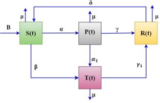
The dynamic model for soil pollution comprises four distinct compartments: susceptible soil areas S(t), polluted soil areas (P), areas subject to necessary remedial treatments (T), and the recovered subclasses (R). Soil contamination typically arises from the presence of excessive heavy metals and plastics. Consequently, the application of both organic and inorganic remedies to the soil treatment (T) class becomes crucial, where certain areas may experience recovery while others might reintroduce contaminants to the susceptible soil due to treatment failures. In the contemporary landscape, there is a notable surge in the utilization of heavy metals in daily activities, leading to a recurrent cycle where previously recovered soil reverts to a susceptible state. In light of the above, the transmission dynamics of soil pollution under treatment measures are given in the compartmental representation illustrated in
Figure 1. This model encapsulates the intricate interplay between susceptible and treated soil areas, offering insights into the complex dynamics of soil pollution and the efficacy of remedial measures.
Figure 1. The schematic diagram for the soil pollution model.
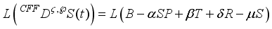
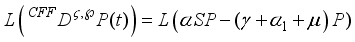
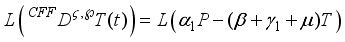
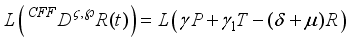
The mathematical model of fractional order is presented as follows,
(1)
with the initial conditions,
(2)
where the parameter and their descriptions are as follows, is the total soil area with
B – recruitment rate of the soil,
- the pollution rate of the soil,
- recovered re-enter to the susceptible rate due to failure of the treatment,
– natural recovered rate,
- remediation rate,
- recovered rate due to treatment,
- recovered re-enter to the susceptible class,
- death rate of all the classes.
3. Existence and Boundedness
For the fractional order system, the existence and uniqueness of solutions in the region , where is considered, where is some positive constant.
Theorem 3.1 If
then for each
there exists a unique solution
of the system (
1) with initial condition
for all
.
Proof: Let us consider the approach of
| [9] | F. Haq, K. Shah, G.-U. Rahman and M. Shahzad, “Numerical analysis of fractional order model of HIV-1 infection of CD4+ T cells”, Computational methods for differential Equations, vol. 5, no. 1, pp. 1-11, 2017. |
[9]
and take
,
The system of equations (
3) is reduced to,
where, , , . For any,
where
Hence
satisfies the Lipshitz condition and so the existence and uniqueness of the solution of fractional order system (
1) with the initial conditions are confirmed.
Theorem 3.2 The system of the fractional order of (
1) in
is non-negative and uniformly bounded.
Proof: The approach used by
| [9] | F. Haq, K. Shah, G.-U. Rahman and M. Shahzad, “Numerical analysis of fractional order model of HIV-1 infection of CD4+ T cells”, Computational methods for differential Equations, vol. 5, no. 1, pp. 1-11, 2017. |
[9]
is followed. Define the function
and
+
Applying the standard comparison theorem for the fractional order given in
| [10] | Fazal Haq and Muhammad Shahzad, “Numerical Analysis of Fractional Order Epidemic Model of Childhood Disease”, Discrete Dynamics in Nature and Society, vol. 2017, Article Id 4057089, pp. 7, 2017. |
[10]
, we have,
where is the Mittag Leffler function. By taking , . Therefore, the solution is uniformly bounded in the region
Now the non - non-negativity of the solution is studied for the fractional order system (
1). In (
1)
Hence the solution of the system is non-negative.
4. Equilibrium and Stability Analysis
There are two equilibrium points exists for the model that are found by equating time derivatives in system (1) to zero as follows,
The two steady states of the model (
1) are given by,
Pollution free equilibrium point:
Pollution extinct equilibrium point:
where , ,
is positive, when (i) and (or)
(ii) and
Basic Reproduction Number (BRN): | [27] | Van den Driessche, Paul, and James Watmough. "Further notes on the basic reproduction number." Mathematical epidemiology (2008): 159-178. |
[27]
The next generation matrix (NGM) is used to find the BRN of the system (1)
Consider,, where
,
where It follows that spectral radius of the matrix is at pollution free equilibrium point . Therefore, the basic reproduction number is,
Theorem: 4.1 If all the eigen values have negative real part then the pollution free equilibrium point
of the system (
1) is locally asymptotically stable.
Proof: From the Matignon condition, we observe that the pollution free equilibrium point is locally asymptotically stable if and only if all the eigenvalues
of the Jacobian
satisfy
The Jacobian matrix of the system (
1) is
(7)
.
Here are the eigenvalues, . Therefore, the eigenvalues . It can be observed that all the eigenvalues of the Jacobian matrix are negative. Hence by using the Matignon condition, we observe that the pollution-free equilibrium is locally asymptotically stable.
Theorem 4.2: The pollution extinction equilibrium point is globally asymptotically stable if and only if and
Proof: Consider the following nonlinear Lyapunov function,
(8)
Take the Lyapunov fractional derivative on both sides,
(9)
After some simplification we obtain,
Finally, we conclude that, , if and only if
The first derivative of a Lyapunov function is instrumental in evaluating the global stability of endemic equilibrium locations. It provides essential insights that can be further enriched by second derivative analysis. While the second derivative informs us about curvature through its sign, the first derivative offers valuable information on disease propagation. Examining the first derivative gives us insights into how the system evolves and spreads over time. Complemented by the second derivative examination, this analysis contributes to a comprehensive understanding of the dynamics and stability of endemic equilibria in disease models.
Taking the second derivative of (
9),
where,
Now, substituting the values of the derivative and rearranging the terms of positive and negative groups, so that we have,
Therefore, we see that,
i. If then
ii. If then
iii. If then
This interpretation explains the model's global behavior with respect to Lyapunov second order derivative.
Lemma 4.1: The given model (1) has no periodic orbits.
Proof: The proof has carried with a Dulac plus Poincare Bendixson theorem as follows:
, where all the parameters are positive.
Hence, from the Dulac principle, we conclude that there is no periodic solution for the given region R.
5. Numerical Approximation
The numerical approximate solution of a system (
1) is obtained using Laplace adomain decomposition method,
Applying Laplace transform on both sides of equation (
1),
Substitute the initial condition
(2) in the above equations,
Now,
(11)
Consider the infinite series,
(12)
Also consider the decomposition of nonlinear terms as follows,
where the decomposition polynomial is defined as follows,
The first three polynomials are,
Substituting above equations in equation (
11),
(14)
Comparing both sides of equation of (
14),
In general,(15)
In general,(16)
In general,(17)
In general,(18)
Taking Laplace inverse transform (LIT) on both sides of the above equations,
Then we have,
Substituting the initial and parameter values, we get the required numerical approximate solution for the equation (
1).
6. Sensitivity Analysis
6.1. Local Sensitivity Analysis
The sensitivity analysis of each parameter of the basic reproduction number with respect to the model statements is performed in order to control the pollution spread through the soil. Sensitivity indices of each parameter in the BRN are calculated to implement the sensitivity analysis
| [27] | Van den Driessche, Paul, and James Watmough. "Further notes on the basic reproduction number." Mathematical epidemiology (2008): 159-178. |
[27]
. The normalized forward sensitivity indices are obtained for different behavior of each parameter in prevalence of pollution transmission. Let M be a normalized forward index variables with respect to the dependent variable
and is defined as follows,
By using explicit form of basic reproduction number, we can find an analytical expression for various parameters of the normalized forward sensitivity indices. The normalized sensitivity analysis at the baseline for each parameter are predicted as follows,
Sensitivity analysis is used to identify the important aspects of different parameters contribution in the results of the basic reproduction number which are based on their uncertainty estimation. Partial rank correlation is the acceleration method to find the statistical influence of the monotonicity relationship between any parameters and the basic reproduction number. The performance sensitivity index is presented in the above calculations which exhibit that positive signs are presented to be very proportionally and highly sensitive to the parameter values of
at the same time those with the negative sign predict less sensitivity to decrease
and other parameters are neutrally sensitive. The positive estimated parameters B and
have been increased (decrease) by 10 % and with the same percentage
is also increased (decrease). The remaining negative parameters decrease (increase) by 10% and the basic reproduction number
by increase (decrease) are estimated in
Table 1.
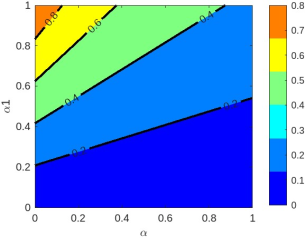
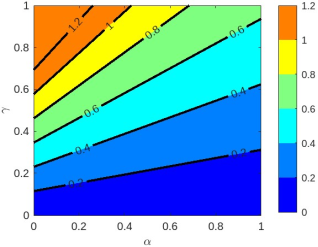
The irrespective effect of the control parameter in basic reproduction number
for the most sensitive parametric representation is illustrated through different contour plots which are shown in
Figures 8 and 9. In addition, the
Figure 7 contour plot shows that increasing the necessary expected remediation rate for the pollution in the soil substance will ultimately reduce the invested amount of secondary pollution number. At the same time, the increased amount of pollution transmission has increased the secondary pollution number. Also, the reduction of pollution transferred into susceptible will decline the basic reproduction number
Figure 8 shows that when the amount gradual increase of recovery rate along with pollution transmission rate acknowledges the reduction of
In addition, the decline rate of transmission in the soil saturation has decreased the BRN.
Table 1. The evaluated parameters of the model (1) at baseline values for the normalized forward sensitivity indices of .
Parameter | Sensitivity indices | Critical values |
B | | 1 |
| | 1 |
| | -0.7741025239 |
| | -0.1557454146 |
| | -1.7824 |
6.2. Global Sensitivity Analysis
The selection of three sampling sites within Coimbatore city, particularly around the 1194 electroplating facilities primarily situated on black soils, underscored the interconnectedness of industrial and agricultural landscapes in the region. The strategic selection of sampling sites near industries and within 1km distance from primary waste and effluent disposal points facilitated a comprehensive assessment of potential soil contamination, highlighting the urgent need for remedial actions to mitigate the adverse effects of heavy metal pollution on both environmental and public health fronts.
| [22] | Sherene T., “Heavy Metal status of soils in Industrial Belts of Coimbatore District, Tamil Nadu”, Nature environment and pollution technology, Vol. 8, No. 3, pp. 613-618, 2009. |
[22]
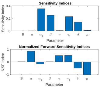
Table 2. Analyzing Sensitivity indices of Cr using the Morris method and Normalized Forward sensitivity indices ().
Parameter | Values 22] | Morris Method | NFSI | Ranges |
B | 0.0234 | 0 | 0.010523 | 0.1-0.3 |
| 0.2 | 0.0026402 | 0.086314 | 0.1-0.5 |
| 0.9 | 0.35434 | -0.16239 | 0.05-0.15 |
| 0.0233 | 0.25161 | 0.007436 | 0.01-0.03 |
| 0.9 | 0.0076827 | 0.50965 | 0.05-0.15 |
| 0.35 | 0.23044 | 0.52066 | 0.05-0.15 |
| 0.05 | 0.14256 | -0.49234 | 0.1-0.3 |
| 0.02 | 0.010727 | -1.0433 | 0.01-0.03 |
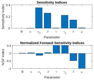
Table 3. Analyzing Sensitivity indices of Ni using the Morris method and Normalized Forward sensitivity indices ().
Parameter | Values 22] | Morris Method | NFSI | Ranges |
B | 0.0234 | 0 | 0.01298 | 0.1-0.3 |
| 0.7 | 0.0026259 | 0.033217 | 0.2-0.7 |
| 0.9 | 0.35209 | -0.13826 | 0.05-0.15 |
| 0.0233 | 0.25952 | 0.04273 | 0.01-0.03 |
| 0.9 | 0.0072494 | 0.52432 | 0.05-0.15 |
| 0.35 | 0.22444 | 0.52874 | 0.05-0.15 |
| 0.05 | 0.14363 | -0.48483 | 0.1-0.3 |
| 0.02 | 0.010451 | -1.0026 | 0.01-0.03 |
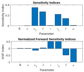
Figure 2. Parameter behaviors in terms Cd transmission using the sensitivity assessment.
Table 4. Analyzing Sensitivity indices of Cd using Morris method and Normalized Forward sensitivity indices ().
Parameter | Values 22] | Morris Method | NFSI | Ranges |
B | 0.0234 | 0 | 0.013388 | 0.1-0.3 |
| 0.9 | 0.002596 | 0.018777 | 0.5-0.9 |
| 0.9 | 0.34795 | -0.13806 | 0.05-0.15 |
| 0.0233 | 0.26974 | 0.053694 | 0.01-0.03 |
| 0.9 | 0.0070178 | 0.52282 | 0.05-0.15 |
| 0.35 | 0.22026 | 0.53043 | 0.05-0.15 |
| 0.05 | 0.14165 | -0.48194 | 0.1-0.3 |
| 0.02 | 0.010788 | -1.0433 | 0.01-0.03 |
Figure 3. Parameter behaviors in terms Ni transmission using the sensitivity assessment.
Figure 4. Parameter behaviors in terms Cr transmission using the sensitivity assessment.
7. Numerical Simulation and Discussion
In this section, the graphical representation of the model is shown for the chosen parameter values and initial values. The parameter values are
,
,
with the initial conditions
We use MATLAB (fde12) to plot the graph of the model (2.1). In
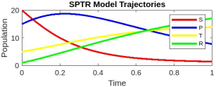
Figure 2,
and fractional order is 0.85. From
Figure 2, we can observe that by increasing the necessary remedial to the polluted soil, there is an increase in recovered soil and a decrease in suspected soil.
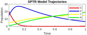
Figure 5. Status of SPTR Model Trajectories for the Cr transmission.
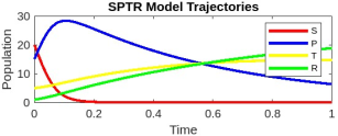
Figure 6. Status of SPTR Model Trajectories for the Ni transmission.
Figure 7. Status of SPTR Model Trajectories for the Cd transmission.
Figure 8. Contour plots of versus communication rate and recovered soil rate due to necessary remedies taken to control the major cause.
Figure 9. Contour plots of versus communication rate and natural recovered rate due to healthy environment ecosystem.
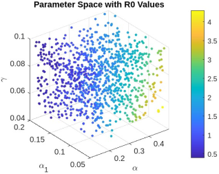
Figure 10. Scatter Plot for different behavior of sensitive indices.
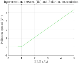
Figure 11. Dynamical effect of secondary pollution number with respect to the pollution cost. Dynamical effect of secondary pollution number with respect to the pollution cost.
8. Conclusion
The paper presents a sophisticated investigation into soil pollution dynamics through the lens of a nonlinear Caputo fractional order eco-epidemic model, specifically designed to capture the complexities of soil contamination. This model, termed SPTR, incorporates four distinct compartments, namely Susceptible soil (S), Polluted soil (P), Treatment or recycling of polluted soil (T), and Recovered soil (R), reflecting the intricate interplay of soil pollution and remediation processes. A pivotal aspect of the study lies in establishing the non-negative and unique existence solution of the model, a fundamental prerequisite for mathematical rigor and applicability. This validation is accomplished utilizing the fixed point theorem, underscoring the mathematical soundness of the proposed model. The investigation extends further to explore the local and global stability properties of both pollution-free equilibrium and pollution extinction equilibrium points within the model. Understanding the stability characteristics is essential for discerning the long-term behavior and resilience of the soil pollution system under various scenarios. To obtain practical insights into the dynamics of the system, the authors employ the Laplace Adomain decomposition method to derive approximate solutions. These solutions offer valuable predictive capabilities, enabling researchers to assess the behavior of the system across different fractional orders and parameter settings. One of the key findings highlighted in the paper pertains to the significance of fractional derivatives over integer derivatives. The flexibility afforded by fractional derivatives provides an additional degree of freedom, allowing for better alignment with empirical data and reduced inaccuracies in modeling soil pollution dynamics. The study emphasizes the importance of implementing effective remediation strategies to mitigate soil pollution. By increasing the treatment rate, the soil recovery process can be expedited, offering practical implications for environmental management and remediation efforts. In addition to theoretical investigations, the paper delves into practical assessments through global sensitivity analysis.
i. This analysis unveils varying concentrations of heavy metals, including total Cr, Ni, and Cd, across different industrial zones and agricultural fields in Coimbatore city, Tamil Nadu. The alarming revelation that Cd levels surpass background metal levels across all industries underscores the urgent need for remedial action to address heavy metal contamination effectively.
ii. Further, the paper represents a comprehensive exploration of soil pollution dynamics, offering theoretical insights, practical implications, and actionable recommendations for environmental stewardship and policy formulation.
Abbreviations
BRN | Basic Reproduction Number |
NGM | Next Generation Matrix |
Replication of Results
No results are presented.
Funding
This paper is not funded by any organization and funding agency.
Data Availability Statement
No underlying data were collected or produced in this study.
Conflicts of Interest
The authors declare no conflict of interest.
References
| [1] |
A. Kilbas, H. M. Srivastava and J. J. Trujillo, “Theory and Applications of Fractional Differential Equations”, Elsevier, Amsterdam, The Netherlands, 2006.
|
| [2] |
Babakhani and V. Daftardar-Gejji, “Existence of positive solutions of nonlinear fractional differential equations”, Journal of mathematical analysis and applications, vol. 278, no. 2, pp. 434-442, 2003.
|
| [3] |
C. F. Li, X, N. Luo, Y. Zhou and J. J, “Existence of positive solution of the boundary value problem for nonlinear fractional differential equations”, Computer and Mathematics with applications, vol. 59, pp. 1363-1375, 2010.
|
| [4] |
D. Kumar and J. Singh, “Application of Homotopy analysis transform method to fractional biological population model”, Romanian reports physics, vol. 65, no. 1, pp. 63-75, 2013.
|
| [5] |
Elhia, M., Balatif, O., Boujallal, L., & Rachik, M. Optimal control problem for a tuberculosis model with multiple infectious compartments and time delays. An International Journal of Optimization and Control: Theories & Applications (IJOCTA), 11(1), 75-91. (2021).
|
| [6] |
Evirgen, Fırat, et al. "Real data-based optimal control strategies for assessing the impact of the Omicron variant on heart attacks." AIMS Bioengineering 10.3 (2023).
|
| [7] |
F. Haq, K. Shah, G. Rahman and M, Shahzad, “Existence and uniqueness of positive solutions to boundary value problem of fractional differential equations”, Sindh Univ. Res. Jour, vol. 48, no. 2, pp. 451-456, 2016.
|
| [8] |
Evirgen, F., Ucar, E., ÖZDEMIR, N., Altun, E., & Abdeljawad, T. (2023). The impact of nonsingular memory on the mathematical model of Hepatitis C virus. Fractals, 2340065.
|
| [9] |
F. Haq, K. Shah, G.-U. Rahman and M. Shahzad, “Numerical analysis of fractional order model of HIV-1 infection of CD4+ T cells”, Computational methods for differential Equations, vol. 5, no. 1, pp. 1-11, 2017.
|
| [10] |
Fazal Haq and Muhammad Shahzad, “Numerical Analysis of Fractional Order Epidemic Model of Childhood Disease”, Discrete Dynamics in Nature and Society, vol. 2017, Article Id 4057089, pp. 7, 2017.
|
| [11] |
Hamou, Abdelouahed Alla, et al. "Analysis and dynamics of a mathematical model to predict unreported cases of COVID-19 epidemic in Morocco." Computational and Applied Mathematics 41.6 (2022): 289.
|
| [12] |
Ipung Fitri Purwanti and Tesya Paramita Putri, “Treatment of Chromium Contaminated Soil using Bioremediation”, AIP Conference Proceeding, 1903, 040008, 2017.
|
| [13] |
Kashyap, A. J., Bhattacharjee, D., & Sarmah, H. K. (2021). A fractional model in exploring the role of fear in mass mortality of pelicans in the Salton Sea. An International Journal of Optimization and Control: Theories & Applications (IJOCTA), 11(3), 28–51.
https://doi.org/10.11121/ijocta.2021.1123
|
| [14] |
Liao, Teh-lu. "Adaptive synchronization of two Lorenz systems." Chaos, Solitons & Fractals 9.9 (1998): 1555-1561.
|
| [15] |
Mukharjee D and Mondal R, “Dynamical analysis of a Fractional Order Prey-Predator system with reserved area”, J Fract Calc Appl 11, 54-69, 2020.
|
| [16] |
Muhammad Rafiq and Javaid Ali,“Numerical Analysis of a bi-model covid-19 SITR model”, Alexandria Engineering Journal, vol. 61, pp. 227-235, 2022.
|
| [17] |
Noor Badshah and Haji Akbar, “Stability analysis of fractional order SEIR model for malaria disease in Khyber Pakhtunkhwa”, Demonstratio Mathematica, vol. 54, pp. 326-334, 2021.
|
| [18] |
Nuri Ozalp and Elif Demiric, “A fractional order SEIR model with vertical transmission”, Mathematics and computer modeling, 54, pp. 1-6, 2011.
|
| [19] |
O. D. Makinde, “Adomain decomposition approach to a SIR epidemic model with constant vaccination strategy”, Applied Mathematics and Computation, vol. 184, no. 2, pp. 842-848, 2007.
|
| [20] |
Ozdemir, Necati, Esmehan Uçar, and Derya Avcı. "Dynamic analysis of a fractional svir system modeling an infectious disease." Facta Universitatis, Series: Mathematics and Informatics (2022): 605-619.
|
| [21] |
S. B. Kurniawan, “Bioprocess of Trivalent Chromium using Bacillus subtilis and Pseudomonas putida”, Department of Environmental Eng., FTSLK ITS Surabaya, 2016.
|
| [22] |
Sherene T., “Heavy Metal status of soils in Industrial Belts of Coimbatore District, Tamil Nadu”, Nature environment and pollution technology, Vol. 8, No. 3, pp. 613-618, 2009.
|
| [23] |
S. S Askar, Dipankar Ghosh, “A fractional order SITR Mathematical model for forecasting of transmission of Covid 19 of India with lockdown effect”, Results in Physics 24, 104067, 2021.
|
| [24] |
Subrata Paul and Animesh Mahata, “Dynamics of SIQR epidemic model with fractional order derivative”, Partial differential equation in applied mathematics, vol. 5, 100216, 2022.
|
| [25] |
V. Lakshmikantham and A. S. Vatsala, “Theory of fractional differential inequalities and applications,” Communications in Applied Analysis, vol. 11, pp. 395–402, 2007.
|
| [26] |
V. Lakshmikantham and A. S. Vatsala, “Basic theory of fractional differential equations,” Nonlinear Analysis: Theory, Methods & Applications, vol. 69, no. 8, pp. 2677–2682, 2008.
|
| [27] |
Van den Driessche, Paul, and James Watmough. "Further notes on the basic reproduction number." Mathematical epidemiology (2008): 159-178.
|
| [28] |
Wu, Jianyong, et al. "Sensitivity analysis of infectious disease models: methods, advances and their application." Journal of The Royal Society Interface 10.86(2013): 20121018.
|
| [29] |
Y. Li, Y. Chen and I. Podlubny, “Stability of fractional-order nonlinear dynamic systems: Lyapunov direct method and generalized Mittag-Leffler stability,” Computers & Mathematics with Applications, vol. 59, no. 5, pp. 1810–1821, 2010.
|
| [30] |
Zhang, Zizhen, et al. "Dynamics of a fractional order mathematical model for COVID-19 epidemic." Advances in Difference Equations 2020. 1(2020): 1-16.
|
Cite This Article
-
-
@article{10.11648/j.ijees.20240902.12,
  author = {Priya Pichandi and Sabarmathi Ayyavu},
  title = {Global Sensitivity Analysis of Soil Pollution Using Fractal Fractional Order Model
},
  journal = {International Journal of Energy and Environmental Science},
  volume = {9},
  number = {2},
  pages = {38-51},
  doi = {10.11648/j.ijees.20240902.12},
  url = {https://doi.org/10.11648/j.ijees.20240902.12},
  eprint = {https://article.sciencepublishinggroup.com/pdf/10.11648.j.ijees.20240902.12},
  abstract = {This research investigates the profound impact of land pollution on soil degradation, stemming from human-made (xenobiotic) chemicals and alterations in soil composition. The framework explains a comprehensive nonlinear fractal fractional order eco-epidemic model, delineating four compartments: Susceptible soil (S), Polluted soil (P), Remediation or recycling of polluted soil (T), and Recovered soil (R). The study rigorously establishes the non-negative and unique existence of solutions using the fixed point theorem while analyzing the local and global stability of equilibrium points under pollution-free equilibrium and pollution extinct equilibrium. Dula’s criterion confirms periodic orbits, while categorizing changes in secondary reproduction numbers provides crucial insights into pollution dynamics, enhancing our understanding of system dynamics. Local and global sensitivity analyses, employing forward sensitivity and the Morris Method, yield essential findings for informed decision-making. Additionally, Adams-Bashforth's method is employed to approximate solutions, facilitating the integration of theoretical concepts with practical applications. Supported by numerical simulations conducted in MATLAB, the study offers a nuanced understanding of parameter roles and validates theoretical propositions, ultimately contributing valuable insights to environmental management and policy formulation.
},
 year = {2024}
}
 Copy
|
Copy
|
 Download
-
TY  - JOUR
T1  - Global Sensitivity Analysis of Soil Pollution Using Fractal Fractional Order Model

AU  - Priya Pichandi
AU  - Sabarmathi Ayyavu
Y1  - 2024/08/15
PY  - 2024
N1  - https://doi.org/10.11648/j.ijees.20240902.12
DO  - 10.11648/j.ijees.20240902.12
T2  - International Journal of Energy and Environmental Science
JF  - International Journal of Energy and Environmental Science
JO  - International Journal of Energy and Environmental Science
SP  - 38
EP  - 51
PB  - Science Publishing Group
SN  - 2578-9546
UR  - https://doi.org/10.11648/j.ijees.20240902.12
AB  - This research investigates the profound impact of land pollution on soil degradation, stemming from human-made (xenobiotic) chemicals and alterations in soil composition. The framework explains a comprehensive nonlinear fractal fractional order eco-epidemic model, delineating four compartments: Susceptible soil (S), Polluted soil (P), Remediation or recycling of polluted soil (T), and Recovered soil (R). The study rigorously establishes the non-negative and unique existence of solutions using the fixed point theorem while analyzing the local and global stability of equilibrium points under pollution-free equilibrium and pollution extinct equilibrium. Dula’s criterion confirms periodic orbits, while categorizing changes in secondary reproduction numbers provides crucial insights into pollution dynamics, enhancing our understanding of system dynamics. Local and global sensitivity analyses, employing forward sensitivity and the Morris Method, yield essential findings for informed decision-making. Additionally, Adams-Bashforth's method is employed to approximate solutions, facilitating the integration of theoretical concepts with practical applications. Supported by numerical simulations conducted in MATLAB, the study offers a nuanced understanding of parameter roles and validates theoretical propositions, ultimately contributing valuable insights to environmental management and policy formulation.

VL  - 9
IS  - 2
ER  -
Copy
|
Download